Lambda Calculus
August 04, 2021

Lambda calculus is a formal system in mathematical logic for
expressing computation based on function abstraction and
application using variable binding and substitution.
Lambda calculus was introduced by the mathematician Alonzo
Church in the 1930s as part of his research into the
foundations of mathematics.
Lambda calculus consists of constructing lambda terms and
performing reduction operations on them.
In the simplest form of lambda calculus, terms are built
using only the following rules:
| Syntax | Name | Description |
|---|---|---|
| x | Variable | A character representing a parameter or a value. |
| (λx.M) | Abstraction | Function definition. |
| (A B) | Application | Applying a function to an argument. |
There also exist some ways to reduce a given lambda expression:
| Syntax | Name | Description |
|---|---|---|
| λx.M[x] → λy.M[y] |
α-conversion | Renaming the bound variables to avoid collisions. |
| (λx.M E) → M[x:=E] |
β-reduction | Replacing the variables with the argument in the body of the abstraction. |
In the next sections we are going further explore the possibilies of this kind of programming language.
An Interpreter is a complex program, so it will be easier if we split the task of parsing and interpreting the given expression into multiple smaller stages:
| Name | Description | |
|---|---|---|
| 1. | Lexer | Turns a sequence of characters (plain text) into a sequence of tokens. |
| 2. | Parser | Takes a sequence of tokens and produces an abstract syntax tree (AST) |
| 3. | Interpreter | Interprets the AST of the source of a program on the fly (without compiling it first). |
Eventually we want to create a function which takes an input string and performs the lexical analysis, the parsing, and the interpreting and returns the reduced AST in the end. It could look something like this:
Attention: The following code snippets are condensed to the bare minimum. You can find the full code on my Github-Page.
A Lexer or sometimes called Tokenizer is a small programm
which takes a sequence of characters (the "source code" of our
λ-Expressions) and turs them into a sequence of predefinded
Tokens.
In addition to analizing and splitting the input-string the
lexer also has some utility-functions which we can later use
to parse the expression.
We also define a Token-class in which we store the type and the possible value of our encountered symbols.
This allows us to tokenize our first string:
As result we get a list of all the tokens in the input string.
This concludes the Lexer and we can now begin parsing
the expression.
A Parser performs an analysis of the given tokens and creates an abstract syntax tree (AST). During parsing it closely follows the rules specified by the given "formal grammar"
Bevore we can start to parse our tokens, we first must specify the grammar the parser is going to follow:
In the following section some of the valid strings this grammar allows are shown:
Now we can write our Parser, which impements the grammar rules specified above:
We also need to define our Node-classes which hold information
about the underlying structure of groups of tokens.
The goal is to create an abstract syntax tree (AST) which
contains all structural informations of the given tokens.
The Node classes already contain some helper functions which
we later need to interpret the AST.
Now we can parse the tokens we previously aquired from the Lexer and create the abstract-syntax-tree:
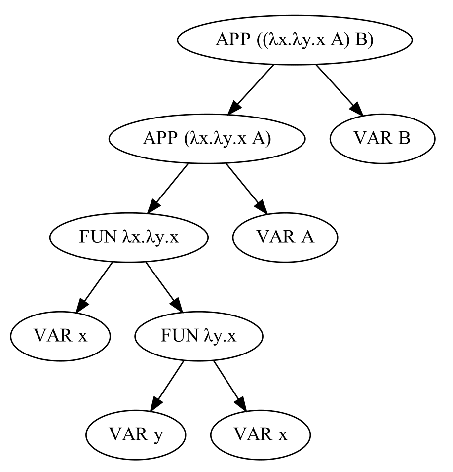
The AST is a Node that has references to other nodes inside
which also refer to their children nodes and so forth.
In this example the AST is an Application Node which contains
another Application Node and a Variable Node. The internal
Application Node contains itself a Function Node that also
contains another Function Node inside.
In the following image you can see a drawing of the AST with
all its sub-nodes.

The Interpreter takes the AST we evaluated bevore and tries to interpet it. In this case, due to the nature of lambda-calculus the interpreter just simplifies the given AST as far as possible.
Now we can put everything together:
Now that we have completed our basic tokenize-parse-interpret system, we can use it to calculate some advanced expressions and and represent features such as boolean logic, arithmetic expressions and datastructures such as lists.
There are no boolean variables in our λ-calculus yet, so we
need to define them:
The standard way of modeling truth values is the following:
| Name | λ-expression | Description |
|---|---|---|
| TRUE | λx.λy.x | Function that takes two parameters, returns the first |
| FALSE | λx.λy.y | Function that takes two parameters, returns the second |
Now we can define the boolean operators:
| Name | λ-expression | Description |
|---|---|---|
| AND | λp.λq.((p q) p) | Evaluates the logical AND between p and q |
| OR | λp.λq.((p p) q) | Evaluates the logical OR between p and q |
If we look at the AND operator, we see that in its body it
evaluates "((p q) p)"
Lets immagine that p is TRUE for now. If we look at the
encoding for the TRUE value, we see that TRUE is just a
function that expects 2 parameters and returns the first one.
The body of the AND operator does exactly this: It "calls" the
TRUE function with the parameters "q" and "p" and returns the
result.
We said that p is TRUE, therefore it will return the first
argument it sees, in this case it will be the value "q".
That makes sense, because if the first parameter to the AND
function is TRUE, the total output depends just on the other
parameter.
In the other case, if we say p is FALSE, it will return the
second argument it receives. In the case of the AND operator,
the second argument is also "p". That means it will always
return itself, which we already defined to be FALSE.
This concludes the AND operator. The OR operator works in a
similar way.
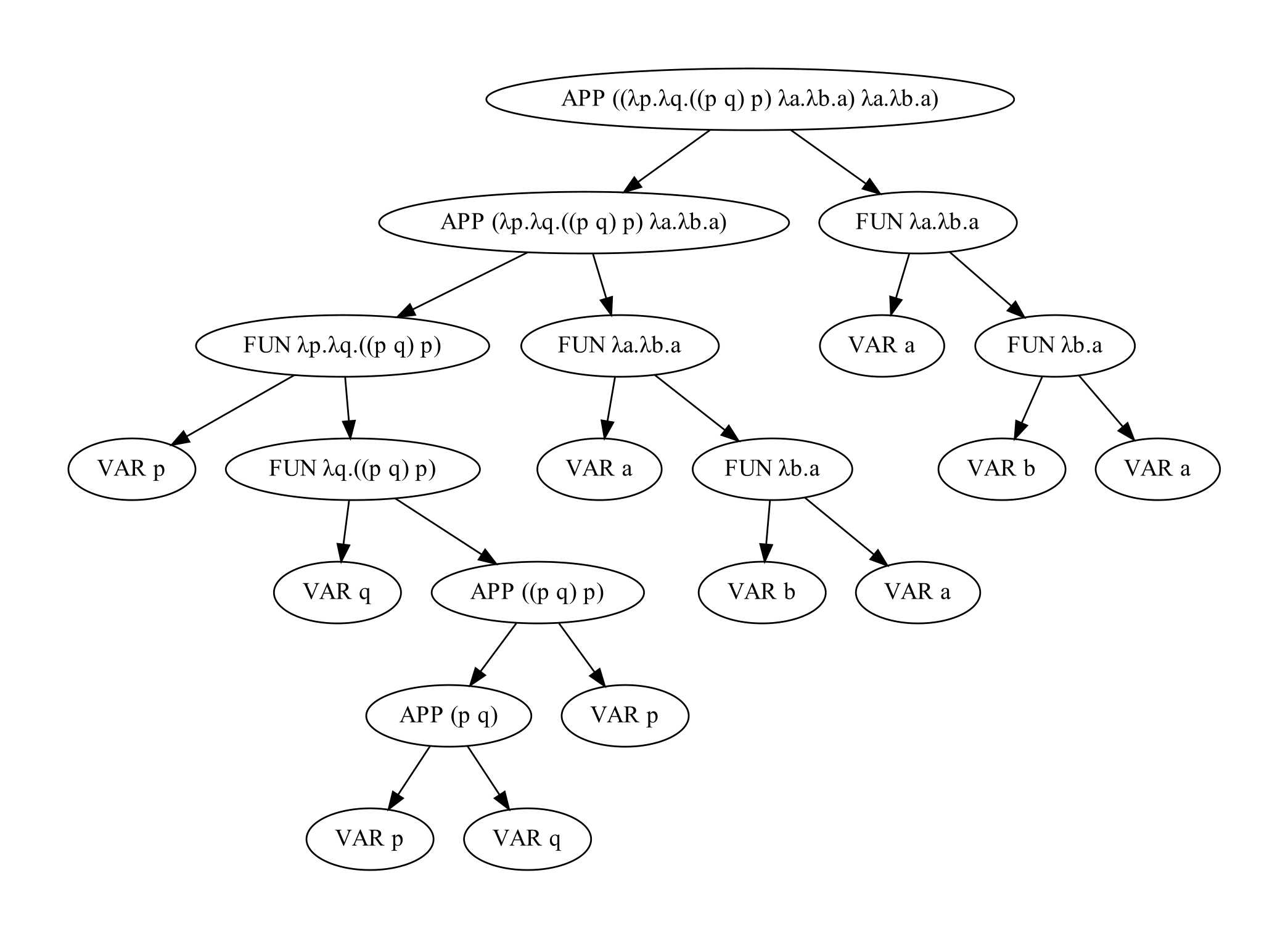
The following code snipet shows the result of such an evaluation:
Here you can see the full AST of this input:

There is also a way to implement numbers in the λ-calculus.
The idea behind these church-numerals are the peano-axioms.
| Name | λ-expression | Description |
|---|---|---|
| ZERO | λf.λx.x | Encodes 0 |
| ONE | λf.λx.(f x) | Encodes 1 |
| TWO | λf.λx.(f (f x)) | Encodes 2 |
| THREE | λf.λx.(f (f (f x))) | Encodes 3 |
| ... | ... | ... |
| N | λf.λx.(fn x) | Encodes n |
We can also define some basic functions:
| Name | λ-expression | Description |
|---|---|---|
| SUCC | λn.λf.λx.(f ((n f) x)) | Evaluates the successor of n |
| PLUS | λm.λn.λf.λx.((m f) ((n f) x)) | Evaluates m+n |
| MULT | λm.λn.λf.(m (n f)) | Evaluates m*n |
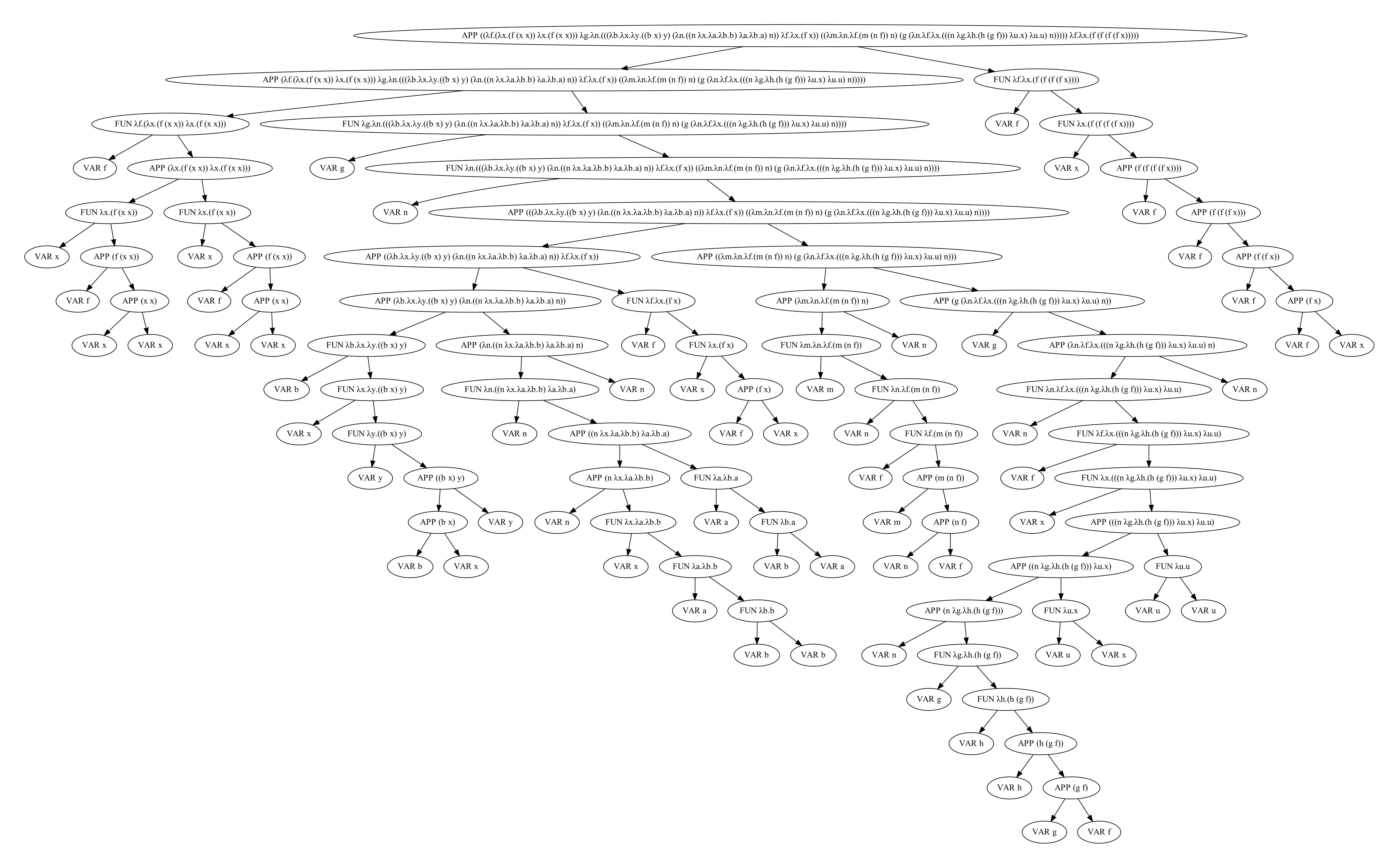
The following code snipet shows the result of such an evaluation:
Here you can see the full AST of this input:

In the λ-calculus a Function cannot call itself, therefore we
need to find another way of representing recursion.
One possibility is a so called "Fixed-point combinator", in
particular the "Y-combinator".
| Name | λ-expression | Description |
|---|---|---|
| Y | λf.(λx.(f (x x)) λx.(f (x x))), | Encodes the Y-combinator |
| FACT_STEP | λg.λn.(((IFTHENELSE (ISZERO n)) ONE) ((MULT n) (g (PRED n)))) | Encodes the non recursive part of the factorial-function |
| FIB_STEP | λg.λn.(((IFTHENELSE ((LEQ n) TWO)) ONE) ((PLUS (g (PRED n))) (g (PRED (PRED n))))) | Encodes the non recursive part of the fibonacci-function |
| FACT | (Y FACT_STEP) | Encodes the factorial-function |
| FIB | (Y FIB_STEP) | Encodes the fibonacci-function |
The following code snipet shows the result of such an evaluation:
Here you can see the full AST of this input:

Is this the best possible implementation? Probably not, however, it is where I am going to leave it for now. I achieved my goal of learning the basics of λ-calculus and created my own little programming to dynamically evaluate λ-expressions.
However, I have also learned that my implementation is slow and inefficient, because, in my implementation, evaluating a result relies on recursiveley renaming all the variables in the subtree. This is very slow, and in general my code is not well optimized.
The code shown above is just a small subset of the actual programm. If you want to take a further look on the project, you can find the full code on my Github-Page.